Summary

In this article, I want to explore one method that allowed Celantur to decrease developer downtime by achieving 20 times the performance of built-in numpy.std() and numpy.mean() algorithms for uint8 images. If you are only interested in the algorithm, feel free to skip the introduction part and jump directly to algorithm.

Introduction

When calculating pixel-wise image differences that we use to compare different iterations of our blurring algorithm, some normalization is required. It can be easily understood using the following example. Let's take a look at two stock images taken from Unsplash anonymised using Celantur’s 2022 and 2023 blurring algorithm.

Let’s now calculate pixel-wise difference between the two:

import cv2
import numpy as np

# Load both images
img1 = cv2.imread("algo_2022.jpg")
img2 = cv2.imread("algo_2023.jpg")
w, h = img1.shape[1], img1.shape[0]

# Calculate absolute pixelwise difference between images
diff = np.sum(np.abs(img1 - img2))
print(f"Absolute difference algo_1 <-> algo_2 is {diff}") 

The resulting absolute image difference is 2,387,317,315, or around 2 billions. This number does not tell us anything yet, but we expect that by comparing more and more images we will probably get some reference values that we can set as a threshold to signal that something changed substantially in our software.

Or can we?

Unfortunately, this number is absolutely useless as a threshold. To check this out one could, for example, try to resize the images:

resized_img1 = cv2.resize(img1, (int(w/10), int(h/10)))
resized_img2 = cv2.resize(img2, (int(w/10), int(h/10)))
diff_resized = np.sum(np.abs(resized_img1 - resized_img2))
print(f"Absolute difference algo_1 <-> algo_2 resized is {diff_resized}")

The output is 23,708,069, or 100 times lower than our previous image case. This means that for the same algorithmic change, we will get a 100-time smaller pixel-wise difference if our test images are 100 times (in terms of number of pixels) smaller. The solution in this case is to divide the total pixel-wise difference by the image size and this is called normalization.

The same story repeats with the image’s brightness and contrast. To achieve the pixel-wise difference metrics that contains more information, each image channel needs to be normalized by it's mean and standard deviation values:

mean_1 = np.mean(img1,axis=(0,1))
std_1 = np.std(img1,axis=(0,1))
img1 = (img1 - mean_1) / std_1 / (w*h)

The process of normalization of an image from the reference dataset takes 1.6 seconds per image, meaning 2 x 1.6 = 3.2 seconds for one comparison and therefore for 1,500 comparisons in total in the testing pipeline it will take 4,800 seconds, or 1 hour and 20 minutes only for normalization. This additional downtime is unacceptable for a developer.

To improve this runtime, we used a combination of a custom C module and a new normalization algorithm. The resulting time for normalization of the image is 0.08 seconds, or 20 times as fast as the native NumPy implementation. It takes only 4 minutes to finish 1,500 comparisons.

C algorithm to improve NumPy

First, we need to find out exactly which subroutine calls are underperforming. For this we used Python profilers together with pyprof2calltree to export the results into KCachegrind. The results can be interpreted only one way: the overwhelming majority of time was spent in numpy.std() and the next bigger time waste was numpy.mean(). Famously, calling C functions from Python code is an expensive task on it’s own, so my first attempt was just to put the whole normalization calculation directly into the C code.

static PyObject* naive_normalization(PyObject* dummy, PyObject* args) {
    PyObject *arg1=NULL;
    PyObject *arr1=NULL;

    // Get the input argument: convert from Python to C
    if (!PyArg_ParseTuple(args, "O", &arg1)) 
        return NULL;

    // Get the first argument as a Numpy array
    arr1 = PyArray_FROM_OTF(arg1, NPY_UINT8, NPY_IN_ARRAY); 
    if (arr1 == NULL)
        return NULL;

    // Get the shape of the array
    npy_intp *shape = PyArray_SHAPE(arr1);
    // Get pointer to the uint8 data 
    npy_uint8 *data = PyArray_DATA(arr1); 

    // Create a new array with the same shape as the input array. It will be returned as the output of the function.
    PyObject* out = PyArray_SimpleNew(3, shape, NPY_FLOAT64); 
    npy_float64* out_data = PyArray_DATA(out);

    // Calculate the mean for each channel using ...
    npy_float64 mean[3];
    for (int i = 0; i < 3; ++i) 
        mean[i] = 0;
    for (int i = 0; i < shape[0]*shape[1]*shape[2]; ++i) {
        int channel = i % 3;
        mean[channel] += (npy_float64) data[i];
    }
    for (int i = 0; i < 3; ++i) 
        mean[i] /= (npy_float64) shape[0]*shape[1];

    // Calculate the standard deviation for each channel using ...
    npy_float64 std[3];
    for (int i = 0; i < 3; ++i) 
        std[i] = 0;
    for (int i = 0; i < shape[0]*shape[1]*shape[2]; ++i) {
        int channel = i % 3;
        std[channel] += (data[i] - mean[channel]) * (data[i] - mean[channel]);
    }

    for (int i = 0; i < 3; ++i) 
        std[i] = sqrt(std[i] / (shape[0]*shape[1]));
    
    // finally, normalize the data
    for (int i = 0; i < shape[0]*shape[1]*shape[2]; ++i) {
        int channel = i % 3;
        out_data[i] = (data[i] - mean[channel]) / std[channel];
    }

    Py_DECREF(arr1);

    return out;
}

The first argument PyObject* dummy in this function is not important to us, since this is dummy argument required for any C function that extends to Python. Actual arguments are passed as the tuple in the PyObject* args argument. First, we transform the Python arguments to an actual C object. Next, we extract the shape of our array and the pointer to its beginning. This is everything we need to work with the input array in C.

Then, we allocate the output array that has the same shape as the input array but has type NPY_FLOAT64, i.e. 64-bit floating point number. Notice that we don’t really need this large precision in practice, but for the sake of the article we wanted that the Python results have a 1-to-1 correspondence to the results obtained with the custom function, which fails to do so for lower precision.

Afterwards, we calculate the mean and standard deviation for each image channel. Standard deviation is calculated using the equation from numpy.std. Finally, we populate the output array, manually decrease the reference count of the input array (to signal Python garbage collector that the array is now under its control) and return the output array.

The results of this simple move from Python to C are quite impressive. In Python, it takes 1.37 seconds, but our C routine needs only 0.3 seconds. Around 4.5 times performance improvement just moving from Python to C!

But we did not want to stop there. Even though it is a substantial improvement, our 80 minute pipeline would take now around 18 minutes to complete. We still wanted to bring this number down so that developers need to wait less for the testing pipeline to finish.

Further improvement of naive algorithm.

To improve on our result even more we need to take a look at what exactly our algorithm is doing. For the sake of simplicity, let's take a look only at the calculation of the mean. Let us further concentrate on only one image channel here, let’s say red.

The red image channel consists of WxH=N pixels, where W and H are width and height of the image respectively. To calculate the mean, we perform N times the sum of the pixel values. The number N may vary substantially from image to image, but we can assume it to be in the order of one million, since this is the smallest image size our clients provide to us and real life photos will almost always be larger than one megapixel.

The pixel values, however, are limited by their precision np.uint8 and therefore there are only 256 possible pixel values. Because this number is much lower than the total number of pixels (at least three orders of magnitude lower) it seems than our sum contains a lot of members that are equal to each other. In principle, it should be possible to calculate the sum much faster using multiplication instead of the summation. We need to know how often each value is encountered in the image, or put differently, we the histogram that describes value distributions in the red channel. This can be easily represented by integer array of size 256:

int red_hist[256];

Then, moving over the channel, we need to fill this array with values:

for (uint8 i = 0; ... iterate over red channel values) 
  red_hist[i]++;

Finally, having this histogram in hand we can calculate the result:

for (int i = 0; i < 256; ++i) {
  red_mean = red_mean + hist[i] * i;
}
red_mean = red_mean / (W * H);

What is even better, this expression easily extends to the standard deviation:

for (int i = 0; i < 256; ++i) {
    red_std = red_std + hist[i] * (i - red_mean) * (i - red_mean);
}
red_std = sqrt(red_std/(W * H));

It is clear that the derived expression must outperform the naive calculation. The (i - red_mean) * (i - red_mean) calculation here must only be performed 256 times, while in the naive calculation it is performed N times. This in turn requires two casts of i from uint8 to float, float subtraction and float multiplication. Logically, this computation should result in better performance. Furthermore, it must perform even better as the size of the image increases.

Here is the full implementation of this code in C:

typedef unsigned long img_index_t; // must contain the largest possible image size

struct mean_std {
    npy_float64 mean;
    npy_float64 std;
};

struct mean_std get_mean_std(npy_uint8* a, img_index_t shift, img_index_t channels, img_index_t size) {
    struct mean_std out;
    out.mean = 0.0f;
    out.std = 0.0f;

    img_index_t denominator = (size/channels);
    img_index_t hist[256];
    for (img_index_t i = 0; i < 256; i++) {
        hist[i] = 0;
    }

    // calculate histogram
    for (img_index_t i = shift; i < size; i+=channels) {
        hist[ a[i] ]++;
    }

    // calculate mean
    img_index_t sum = 0;
    for (int i = 0; i < 256; ++i) 
        sum = sum + hist[i] * i;
    out.mean = ((npy_float64) sum)/((npy_float64) denominator);
    
    //calulate standard deviation
    for (int i = 0; i < 256; ++i) 
        out.std = out.std + ((npy_float64) hist[i]) * (i - out.mean) * (i - out.mean);
    out.std = sqrt(out.std/denominator);

    return out;
}

We pass into this function an image size img_index_t size, number of image channels img_index_t channels and current channel img_index_t shift. Notice that we use custom unsigned integer type for iterating over the images img_index_t that is selected to be able to index the maximum image size we can pass to this function.

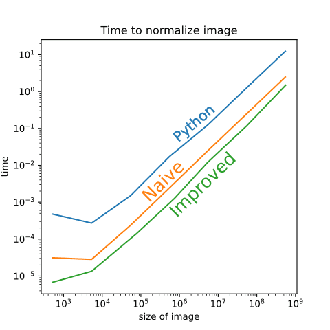
The algorithm we just developed is 2.0 - 5.0 times faster than naive C algorithm, depending on the image size. Since the performance gain seemed to be image dependent, we also tried to compare different image sizes to check whether our algorithm is faster acroos the board or we got lucky with input data:

Which cemented the conclusion that our algorithm is better in all circumstances.

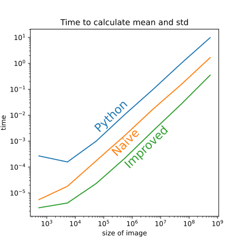
What is also interesting in this figure is that our improved method generally displays the same dynamic as the naive-C and Python implementation when the size of the image increases. This makes sense, since all of them contain the step of actual normalization that does not improve if we speed up calculations of standard deviations and means. For the company this is the the only metric that matters, but for its ambitious employees what matters is how much they could beat the NumPy in these calculations. Let’s now look at how much our new calculation beats NumPy’s std and mean methods.

As one can see from this plot, the time it takes to calculate the mean and std has an order of magnitude difference between Python, naive-C, and improved-C. These are already great results, since if somebody is interested only in e.g. standard deviation, it can be calculated with this method hundred times faster than in the NumPy. But can we improve the actual normalization process, that includes populating the output array even more?

Further improvement of normalization.

Now, having this histogram tool, we can try to further improve the performance. I will continue to explain everything using only the red channel array here, but the generalization to more channels is trivial. When calculating the normalized value of a pixel, we need to perform the following computation:

for (int i = 0; i < size; ++i) {
    arr_out[i] = (arr_in[i] - mean) / std;
}

As previously, there are only 256 possible values assigned to arr_out[i], but its value is calculated size-times. Since size is normally much larger than 256, we could probably substantially improve the computation speed by precalculating all 256 possible values:

void normalize_fast(const uchar* arr_in, float* arr_out, int size, float mean, float std) {
    float cache[256];
    for (int i = 0; i < 256; ++i) {
        cache[i] = (i - mean) / std;
    }

    for (int i = 0; i < size; ++i) {
        arr_out[i] = cache[arr_in[i]];
    }
}

In essence, now instead of size-times float divisions, substractions, and assignments we need to do only 256 float divisions and substractions! Afterwards, size assignments are performed. As before, logically this code must perform better, but in this application we were in for huge disappointment. If we profile it using

valgrind --tool=callgrind --dump-instr=yes --simulate-cache=yes --collect-jumps=yes ./our_exe

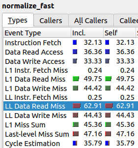
We will see that “improved” algorithm is actually taking twice as long! But luckily for us, the problem of new algorithm can already be detected in the output of the profiler.

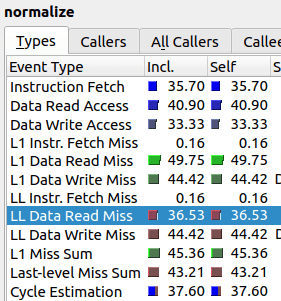
As one can see, the value “LL Data Read Miss” is twice as high, which means the relative amount of last level cache misses is much higher for the improved algorithm than for the original. It seems that our “improved” algorithm spends majority of its time trying to communicate to RAM instead of actually performing computations.

In other words, the nested array subscription structure that we have in the improved algorithm cannot contain both arr_in[] and cache[] in its cache. As we can see from the initial algorithm, just the call arr_in[i] results in 37% cache misses. Then, in the improved algorithm, we try to access cache[ array[i] ] which results most of the time in yet another cache miss, i.e. total of two cache misses. Roughly speaking, this is the reason why the second algorithm has almost twice as much cache misses at 63%.

Technically, there are ways out there to “reserve” CPU space in the cache and probably our algorithm could ran faster, but this would take too much time for the simple normalization task we wanted to perform in our CI/CD and to get more performance it will be much easier to parallelize the image normalization process. If the reader have some simple solution to that issue, you are welcome to write us.